The goal of Project Neuron is to get in one place some cute bits I come up with about Aritificial Neural Networks (ANNs) and related stuff.
Some of them are observations left out from books, others ideas I come up with related to classification.
I'll try to not use expressions as training, learning, excitation, inhibition and such because I don't want to introduce unnecessary noise.
I'm not sure about what prerequisites you need to read this stuff, I would say some High School mathematics, but definitely College mathematics
like Linear Algebra and Multi-variable Calculus would come in handy.. what I can say for sure is that you don't need to know any Python library or whatever.
This is not a place to install numpy and let your computer use it, this is a place to look at ANNs from a perspective different than the traditional.
There will be, however, code, after all I'm a Computer Scientist :) But this code will be in Javascript..
Javascript you ask? Yeah, because I had to learn it to get this site up and running.. so I just might as well keep using it :)
Rossenblatt's perceptron was the first neural network.
It is described at different depths in the literature (Haykin 2009, Aggarwal 2023, Theodoridis and Koutroumbas 2009, Bishop 1997) and also omitted in some (Kneusel 2022, Jentzen et al. 2023). If you want to go practical maybe you skip it, as the perceptron is not considered too powerful.
If it is not practical then why devote time to it? Well, 1) it gives you insight into how ANNs evolve and what actually is going on under the hood
2) you discover relationships that you may be unaware of
3) it develops your understanding of more complicated approaches and
4) it is fun.
So, without further due, let us start.
The perceptron is defined as a small algorithm depicted as the signal-flow graph:

The data originates at the square nodes and travels in the direction of the arrows, at $v$ the data gets aggregated and passed on to the function $\phi$.
The values $x_1,\ldots,x_m$ are variables (inputs) and the values $1,b,w_1,\ldots,w_m$ are constants.
That is, in its most general form, the signal-flow graph depicts the function composition $\phi(v(f_0(1,b),f_{1}(x_1,w_1),f_{2}(x_2,w_2),\ldots,f_{m}(x_m,w_m)))$.
Each $f_i$ is a function from $R^2$ into $R$ that combines the constant $w_i$ with the variable $x_i$; where $R$ is the set of real numbers.
The function $v$ is a function from $R^{m+1}$ into $R$ and finally $\phi$ is a function from $R$ into $R$.
Typically the functions $f_i$ are the product of real numbers and the function $v$ is a sum of real numbers.
The $\phi$ function however, takes many forms, from the identity up to a probability function.
In the perceptron, the signal-flow graph shows the calculation of $\displaystyle{\phi(\sum_{i=1}^{m}{w_ix_i}+b)}$.
The sum $\displaystyle{\sum_{i=1}^{m}{w_ix_i}}+b$ can be rewritten as $\vec{w}^T\vec{x} + b$ if we define $\vec{w} = (w_1,\ldots,w_m)$ and $\vec{x} = (x_1,\ldots,x_m)$ (Haykin 2009, Theodoridis and Koutroumbas 2009).
However, the matrix product $\vec{w}^T\vec{x}$ is the dot product $\vec{w}\cdot\vec{x}$ disguised as a matrix product.
Therefore, we can rewrite the perceptron function simply as $\displaystyle{\phi(\vec{w}\cdot\vec{x} + b)}$.
The equation $\vec{w}\cdot\vec{x} + b = 0$ describes an hyperplane on the $m$ dimensional space such that $\vec{w}$ is perpendicular to the hyperplane and the perpendicular distance from the origin to the hyperplane is $|\frac{b}{||w||}|$.
The perceptron training algorithm assumes the data is separable by an hyperplane, that is, there exists a plane such that the points of one class lay on one side of the hyperplane and points of the other class on the other.
Therefore, in the perceptron, the function $\phi$ determines on which side of the hyperplane the point lays.
Typically this function is the sign function, also known as hard limiter. (Haykin 2009)
The function $\mathrm{sign}$ returns $1$ when the argument is positive and $-1$ when it is negative or zero.
To adjust the hyperplane, the perceptron training algorithm extends the vector $\vec{w}$ as $\vec{w'}=(b,w_1,\ldots,w_m)$ and the input vector $x$ as $x'=(1,x_1,\ldots,x_m)$.
This changes the perceptron function to: $\phi(\vec{w}\cdot\vec{x} + b) = \phi(\vec{w'}\cdot\vec{x'})$.
The perceptron incorrectly classifies a vector $\vec{x}$ if and only if $c=1$ and $x$ belongs to the second class or $c=-1$ and $x$ belongs to the first class, where $c=\phi(\vec{w'}\cdot\vec{x'})$
When the perceptron incorrectly classifies a vector $\vec{x}$, the extended weights vector is adjusted as $\vec{w''}=\vec{w'}-c*\vec{x'}$.
The training process is iterative, each vector in each class is tried until the weights vector is no longer adjusted.
         //$k$ is the number of vectors in both classes
         //$\mathrm{class}(\cdot)$ returns the class of the vector
         //$\mathrm{extend}(\cdot)$ extends the vector
        $\vec{w_i'} = x_0'$
        $\vec{w'} = \vec{w_i'}$
        $i = 1$
         while(true){
            $x_i'=\mathrm{extend}(x_i)$
            $c=\phi(\vec{w'}\cdot\vec{x_i'})$
             if($c$!=$\mathrm{class}(x_i)$)
                $\vec{w'}=\vec{w'}-c*\vec{x_i'}$
            $i=(i+1)\, \mathrm{mod}\, k$
             if($i$ = 0){
                 if($\vec{w'}$ != $\vec{w_i'}$){
                    $w_i' = w'$
                     continue
                 }
                 break
             }
         }
One of the first things we notice in the perceptron training algorithm is that the bias is not directly updated.
The reason for this is that when the vectors (input and weights) are extended to a higher dimension, the bias is expressed as a coordinate and adjusted like any other weight.
For the moment I want to keep things simple and omit a discussion about the bias and assume the classes are separable by a hyperplane passing thru the origin.
Furthermore, I will restrain the discussion to vectors on the plane ($R^2$) and in the space ($R^3$).
The next couple of images show both types of weights corrections for vectors on the plane.
The first shows the case where the point is assigned the second class but belongs to the first.
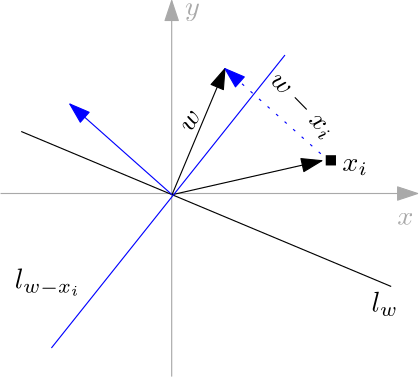
The second image shows the inverse case.
In both images the blue vector (arrow) is the corrected weight and the blue line the induced separating line.
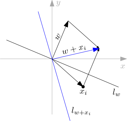
If we make a small mental exercise In both cases we can see that the bigger the difference between the
The bias is an important part of the perceptron.
It allows the hyperplane to move away from the origin.
That property combined with the rotation of the hyperplane makes possible for the perceptron to find a separating hyperplane.
Consider the following example, the points of the first class are disks and the points of the second class are solid squares.

focus on adjusting $\vec{w}$ and leaves the bias $b$ untouched, this is because if the data is separable by an hyperplane, then a translation of the coordinate system can be found such that $b = 0$ and the hyperplane $\vec{w}\cdot\vec{x}$ separates the data.
Therefore, we will restrict to $b=0$.
Hence the perceptron function becomes $\displaystyle{\phi(\vec{w}\cdot\vec{x})}$. and we will take the $\mathrm{sgn}$ function as $\phi(\cdot)$.
Therefore we have $\phi(\vec{w}\cdot\vec{x}) = \mathrm{sgn}(\vec{w} \cdot \vec{x})$.
The dot product between two vectors $\vec{a},\vec{b}$ is defined as $\vec{a} \cdot \vec{b} = \frac{\cos(\theta)}{\left \Vert \vec{a} \right \Vert * \left \Vert \vec{b} \right \Vert}$ where $\theta$ is the angle between $\vec{a}$ and $\vec{b}$.
The sign of $\vec{w}\cdot\vec{x}$ is determined by the cosine of $\theta$ because the norm of a vector is always positive or zero.
As we noted before, the sign of the dot product depends on the cosine of the angle between them so the classification is based on the angle between the weights vector and the data vector.
When is this positive?
To help us recall this, the next figure shows the unit circle. In the unit circle, the $(x,y)$ coordinates of a point on the circle correspond to the cosine and sine of the angle of the vector.

That is: $(x,y) = (\cos(\theta),\sin(\theta))$, so, the cosine is positive if the angle $\theta$ is within the interval $(-\frac{3\pi}{2},\frac{\pi}{2})$.
To easily see the class separation induced by the vector $\vec{w}$ the coordinate system can be rotated counter-clock wise (via a rotation matrix) until the coordinate axis $x$ is over $\vec{w}$.
On this rotated coordinate system, everything in the direction of $\vec{w}$ belongs to one class and everything in the opposite direction of $\vec{w}$ to the other.
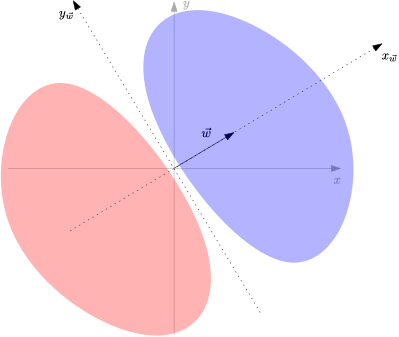
So, we can describe in few words what does it mean to train a perceptron: To point $\vec{w}$ in the right direction :)
There are two main flavors to adjust $\vec{w}$, one is on a failed classification basis (Haykin 2009).
In it, each time the perceptron fails to classify a data point, $\vec{w}$ is updated and the adjustment continues.
The other way to adjust $\vec{w}$ is to test all data points and aggregate all the individual adjustments that would take place in the first method and apply them to $\vec{w}$ (Theodoridis and Koutroumbas 2009).
Both methods find a solution, but not necessarily the same solution.
The next example illustrates this difference.
These are some bits to implement a perceptron and a trainset in (bare) Javascript.
We start extending the Array class to perform usual vector operations: get the norm, the unit vector, dot product, sum and scalar product.
        class Vector extends Array {
           constructor(vector, ...rest){
	      ...
           }
           get norm(){
	      let ss = 0
	      for (let i = 0; i != this.length;i++){
	         ss += this[i]*this[i]
	      }
              return Math.sqrt(ss)
           }
           get unitVector(){
	      let n = this.norm
	      let uv = new Vector()
	      for (let i = 0; i != this.length;i++){
	         uv.push(this[i]/n)
	      }
	      return uv
           }
           // Dot product
           dProduct(vector){
  	      let dp = 0
	      for (let i = 0; i != this.length;i++){
	         dp += vector[i]*this[i]
	      }
	      return dp
           }
           sum(vector){
	      let s = new Vector()
	      for (let i = 0; i != this.length;i++)
	         s.push(vector[i] + this[i])
	      return s
           }
           //Scalar product
           sProduct(scalar){
	      let s = new Vector()
	         for (let i = 0; i != this.length;i++)
	            s.push(scalar*this[i])
	      return s
           }
        }
The Neuron class is self-explanatory, it evaluates the neuron and corrects the weights.
        class Neuron {
        ...
           //Applies the given corrections to the weights
           //classification must be +1 or -1
           //corrections is an array of floats
           correct(classification, corrections){
	      let cc = corrections.sProduct(classification)
              this.weights = this.weights.sum(cc)
           }
        }
The Trainset class holds vectors for training or testing.
It implements an iter method to iterate over k vectors of a given class in-order.
The training of a neuron is then implemented as iterating a training function over the vectors of both classes.
When the vector is misclassified, a correction is performed (Haykin 2009).
Randomly selecting vectors to train a neuron is not necessary, therefore it is not implemented.
        class Trainset {
           constructor(dimension){
	      this.dimension = dimension
	      this.class1 = []
	      this.class2 = []
           }
           ...
           //Iterates a function over k vectors of the given class
           iter(classN, k, f){
	      let tclass = null
	      if(classN == 1)
	         tclass = this.class1
	      else
	         tclass = this.class2
	      if (k > tclass.length)
	         k = tclass.length
	      for (let i = 0; i != k; i++)
	         f(tclass[i])
           }
           //Trains the neuron with c1_train_count vectors of class1 and
           //c2_train_count neurons of class 2 using eta_n = 1
           train_neuron(neuron, c1_train_count, c2_train_count){
	      let c = 1
	      let ts = this
	      console.log("Initial neuron n: " + n.weights)
	      const train = function(v) {
	          console.log("Training with v = " + v + " class: " + c)
	          if (!ts.eval_neuron(neuron,c,v))
		      neuron.correct(c,v)
	          console.log("Resulting neuron: " + n.weights)
	      }
	      this.iter(c,c1_train_count,train)
	      c = -1
	      this.iter(c,c2_train_count,train)
            }
        }
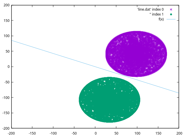
The next image shows a dataset composed of two disks with the same radius.
Both disks are spread at the same distance from a straight line to ensure they are linearly separable.
The interior of the disks are filled by random points.
The straight line in the image is a classification line of a neuron.
Copyright Alfredo Cruz-Carlon, 2025